Contents
- Transformer I
- Transformer II (cont’d)
이번 강의에서는 현재 NLP 연구 분야에서 가장 많이 활용되고 있는 Transformer(Self-Attention)에 대해 자세히 알아봅니다. Self-Attention은 RNN 기반 번역 모델의 단점을 해결하기 위해 처음 등장했습니다. RNN과 Attention을 함께 사용했던 기존과는 달리 Attention 연산만을 이용해 입력 문장/단어의 representation을 학습을 하며 좀 더 parallel한 연산이 가능한 동시에 학습 속도가 빠르다는 장점을 보였습니다
Further Reading
Transformer I
과거 Attention is all you need 논문을 포스팅했던 적이 있지만, naver boostcamp 과정을 수강하면서 다시 한 번 등장한 transformer에 대해 포스팅 하려고 한다. 지난번엔 논문의 흐름에 따라 설명을 진행했다면 이번 포스팅에서는 조금 더 실질적이고 사용적 측면에서 바라보며 포스팅할 예정이다.
RNN: Long-term dependency

- “I go home”이라는 문장을 받았을 때 매 time step $t$마다 $x_t, h_{t-1}$을 받아서 $h_t$를 만들어낸다.
- 그림에서 왼쪽에서 오른쪽 방향으로 가며 계산되는 hidden state를 encoding하게 된다.
- Attention 연산을 한다해도, 뒤로 갈수록 먼저 입력된 단어 “I”는 희석되게 된다.
Bi-Directional RNNs

- Vanilla RNN의 단점을 보완하기 위한 방식으로 제안된 Bi-directional RNN은 역방향으로도 한번 더 진행해오면서 양방향에서의 encoding 벡터를 학습한다.
- 양방향으로 진행되는 Forward RNN과 Backward RNN 모듈을 병렬적으로 만들고 특정한 timestep에서의 hidden state vector를 concatenate함으로써 두 배의 사이즈로 만들어진 encoding vector를 만든다.
Transformer: Long-Term Dependency

- Transformer의 attention 연산은 self-attention으로써, 기존 attention에서 encoder와 decoder의 입력 벡터가 달랐던 것과 달리 같은 hidden state vector를 사용한다고 생각하면 된다.
- 즉, 그림에서 $x_1$은 decoder hidden state vector임과 동시에 encoder hidden state vector set인 $[x_1, x_2, x_3]$중 하나라고 생각할 수 있다.
- 그러면 첫 번째 timestep을 기준으로 $x_1$은 $[x_1, x_2, x_3]$ 세 encoder hidden states 들과 내적을 통해 attention score를 계산하게 되고, 이는 $h_1$으로 계산될 수 있을 것이다.
- 이러한 방식으로 $h_2, h_3$를 구하게 되는 큰 틀에서의 방식을
Self-Attention이라고 부른다. - 하지만, 일반적인 방식으로 계산하게 된다면 당연하게도 자기 자신과의 내적이 큰 비중으로 할당되게 되고, self-attention module의 output인 $h_{1,2,3}$는 자기 자신에 대한 가중 평균이 높게 잡히게 될 것이다.
- 따라서 이러한 문제를 개선하고자 Transformer에서는 확장된 방식의 attention module을 사용한다.
Query, Key, Value Vectors
Query vector: encoder-decoder 구조에서 decoder hidden state vector에 해당하는 vector를 의미한다. 즉, 현재 timestep $t$에서 계산할 주체가 되는 vector.Key vector: query vector와 내적을 하게 될 각각의 재료 벡터를 의미한다. 즉, encoder-decoder 구조에서 encoder hidden states인 $h_{1,2,3}^{(e)}$를 의미한다.Value vector: 계산된 가중치(attention score)를 가중 평균해서 그 비중을 가중해주기 위해 곱해주는 원래 벡터

- $q_1\cdot k_1$, $q_1\cdot k_2$, $q_1\cdot k_3$를 통해 [3.8, -0.2, 5.9]의 vector를 얻게된다.
- 이는 softmax를 통과하여 [0.2, 0.1, 0.7]이 된다.
- 이렇게 나온 결과는 [$v_1, v_2, v_3$]과 pairwise product 연산을 진행하게된다.
- 결과적으로 $h_1=0.2v_1+0.1v_2+0.7v_3$가 된다.
이러한 방식으로 연산되기 때문에, 자기 자신에 대한 self-attention 연산을 하여도 그 크기가 높지 않게 된다.
Operation process in self-attention

- 실제 작동은 위와 같은 행렬 연산에 의해서 진행된다.
- Embedding된 input $X$는 $W^{Q,K,V}$와의 행렬곱을 통해 $Q,K,V$로 구성된다.
- $Q,K,V$의 각 행은 $X$의 각 행, 즉 각 토큰에 해당하는 vector가 된다.
이 같은 방식을 통해 먼 단어간의 관계 및 유사도를 이전 모델과는 달리 손쉽게 파악할 수 있다.
Transformer: Scaled Dot-Product Attention
- Inputs : a query $q$ and a set of key-value $(k, v)$ pairs to an output
- Query, key, value, and output is all vectors
- Output is weighted sum of values
- Weight of each value is computed by an inner product of query and corresponding key
- Queries and keys have same dimensionality $d_k$, and dimensionality of value is $d_v$
- Value vector는 마지막에 계산된 가중평균을 곱하는 역할만을 하기 때문에 차원의 크기가 Query, Key vector들과는 달라도 상관이 없다.
-
즉, input은 하나짜리 query 벡터 $q$와 $K, V$가 된다.
-
ans it becomes : $A(Q, K, V) = softmax(QK^T)V$.

논문에서의 Transformer 구현 상으로는 동일한 shape으로 mapping된 Q, K, V가 사용되어 각 matrix의 shape은 모두 동일하다.
Problem
- As $d_k$ gets large, the variance of $q^Tk$ increases
- query와 key vector의 차원이 커질수록 해당 내적에 참여하는 dimension 역시 커지게 되고 이때의 분산은 점점 커지게 된다.
- Some values inside the softmax get large
- The softmax gets very peaked
- Hence, its gradient gets smaller
Solution
- Scaled by the length of query / key vectors:
- \[A(Q, K, V) = softmax(\frac{QK^T}{\sqrt{d_k}})V\]
- $\sqrt{d_k}$로 나눠줌으로써 scaling을 시켜준다.

Transformer II (cont’d)
Transformer(Self-Attention)에 대해 이어서 자세히 알아봅니다.
Further Reading
- Attention is all you need, NeurIPS’17
- Illustrated Transformer
- Annotated Transformer
- Group Normalization
Further Question
- Attention은 이름 그대로 어떤 단어의 정보를 얼마나 가져올 지 알려주는 직관적인 방법처럼 보입니다. Attention을 모델의 Output을 설명하는 데에 활용할 수 있을까요?
Transformer: Multi-Head Attention
여러 버전의 head를 병렬적으로 만든 뒤 여러번 수행하여 위험 부담(?)을 줄인다.
- The input word vectors are the queries, keys and values
- In other words, the word vectors themselves select each other
- Problem of single attention
- Only one way for words to interact with one another
- Solution
- Multi-head attention maps $𝑄, 𝐾, 𝑉$ into the $ℎ$ number of lower-dimensional spaces via $𝑊$ matrices
- Then apply attention, then concatenate outputs and pipe through linear layer

-
Example from illustrated transformer
-
각 헤드별로 self-attention 연산을 수행한다.

-
Head별로 계산된 context vector를 concatenate한다.


-
single attention module의 아웃풋과 동일한 사이즈를 위해 적절한 가중치 matrix를 곱해준다.

-
per-layer complexity
-
Maximum path lengths, per-layer complexity and minimum number of sequential operations for different layer types
- $n$ is the sequence length
- $d$ is the dimension of representation
- $k$ is the kernel size of convolutions
- $r$ is the size of the neighborhood in restricted self-attention

Transformer: Block-Based Model
각 Block은 두 개의 sub-layers를 지닌다.
- Multi-head attention 모듈
- Two-layer feed-forward NN(with ReLU)
그리고 이 두 개의 모듈은 모두 Residual connection과 layer normalization 스텝을 거친다
- $LayerNorm(x+sublayer(x))$
Residual connection

- residual connection은 그림에서와 같이 입력 벡터를 attention layer를 통과한 output에 다시 더해주는 방식이다
- 이를 통해 얻을 수 있는 효과는 온전히 input vector가 attention layer를 통과한 뒤의 결과만을 반영한다는 점이다.
- 예를들어 input vector [1, -4]가 일반적인 attention module을 통과한 뒤 [2, 3]이 되었다고 가정하면, residual connection을 통해 [3, -1]의 벡터를 만들게한다. 이는 학습과정에서 온전히 attention module의 역할이 [2, 3]의 벡터를 만들게끔 유도하는 역할을 한다.
- 이 과정을 통해 gradient vanishing 문제를 해결하고, 학습이 안정될 수 있도록 한다.
Layer Normalization
학습 도중 샘플의 분포를 normalization 해주는 다양한 방식이 존재한다.
Layer normalization changes input to have zero mean and unit variance, per layer and per training point (and adds two more parameters)


차이는 있지만, 각 샘플들의 평균을 0, 분산을 1로 만들어주는 과정이다. 이 과정은 Neural network의 특정 node에서 원하는 만큼의 값을 가지도록 조절할 수 있게 해준다.
어쨌든 다양한 normalization중 우리가 볼 Layer normalization은 두 가지 step으로 구성된다.
-
Normalization of each word vectors to have mean of zero and variance of one.
-
Affine transformation of each sequence vector with learnable parameters

- thinking과 machines라는 단어가 각각 4차원의 vector로 표현 되었을 때, word별로 특정 layer에서 발견되는 4개의 node의 값들을 모아서 평균과 표준편차를 모아서 각각 평균과 표준편차를 0과 1로 만들어준다.
- 그러면 이 표준화 작업을 거친 vector의 값들은 바뀌게 된다.(그림에서
2번째) - 이렇게 변환된 vector를
Affine transformation하여 결과로 도출되게 된다.
이렇듯 layer normalization을 거치면서 우리가 원하는 평균과 분산을 주입할 수 있게 된다.
Transformer: Positional Encoding
RNN 계열의 모델은 time step에 따른 input의 순서가 자연스레 정해지게 된다. 하지만, token(word)의 상대적 순서를 알려주는 구조가 없는 transformer에서는 이를 위한 구조가 필요하기에 사용된 방법이 positional encoding이다. 이 내용은 본 블로그의 이전 포스팅에 작성하였기에 생략하도록 한다.

Transformer: Warm-up Learning Rate Scheduler
학습을 조금 더 빠르게 하고, 최종 수렴 모델의 성능을 향상시키기 위한 방식으로써 고정된 learning rate를 사용하는 것이아니라 학습이 진행됨에 따라 lr을 변경시키는 방식이다.
-
Learning rate = \(d_{model}^{−0.5}\cdot min(\#step^{-0.5}, \#step\cdot warmup\_stps^{-1.5})\)

Transformer: Encoder Self-Attention Visualization
-
Words start to pay attention to other words in sensible ways

Colab link에 가면 visualization에 대한 tutorial을 시도해볼 수 있다.
- 좌측상단 “드라이브로 복사” 클릭 후 기존창 닫고 새로 열린창에서 실행
Transformer: Decoder
-
Two sub-layer changes in decoder
-
Masked decoder self-attention on previously generated outputs:

-
Encoder-Decoder attention, where queries come from previous decoder layer and keys and values come from output of encoder

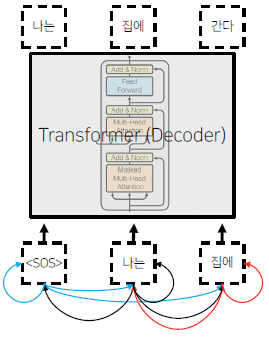
Input과 비슷하게, Output을 shifted right하여 입력한다. 예를 들어보자.
- Input : ‘I go home’
- Output : ‘<SOS> 나는 집에’ 로 입력 sequence로 주어진다.
- ground truth : ‘나는 집에 간다’
이와 같은 방식으로 shifting된 output을 입력으로 준다.(seq2seq에서 decoder input과 같은역할)
Transformer의 Decoder에는 총 2개의 attention module이 있다.
- Masked Multi-head attention
- Multi-head attention
Multi-head attention(Decoder)

위 그림의 빨간색 사각형 부분의 Multi-Head Attention 구조는 Encoder의 multi-head attention module과 구조상으로는 동일하다. 단, 차이점이 있다면 입력으로 들어오는 Q, K, V 벡터가 다른데, 그림에서 볼 수 있듯 두 개의 화살표는 encoder로부터 들어오고, 한 개의 화살표는 아래 Masked multi-head attention module로부터 온다.
Query 벡터는 Masked multi-head attention으로부터 오고, Key 벡터와 Value 벡터는 학습된 상태로 Encoder에서 들어온다.
특히, Masked multi-head attention으로부터 나온 Residual connection은 decoder의 input으로부터 온 query값과 encoder에서 넘어온 벡터를 결합하게 해주는 역할을 할 것이다.
최종적으로 각 벡터의 출력은 FFN와 softmax layer를 거친 뒤 predict 되고, 이는 ground truth와 비교하여 back prop.을 계산하게 된다.
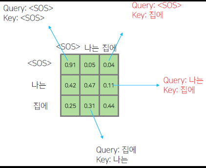
Masked Multi-Head attention(Decoder)
- Those words not yet generated cannot be accessed during the inference time
- Renormalization of softmax output prevents the model from accessing ungenerated words
Decoder의 첫번째 input이 들어온 뒤의 multi-head attention layer로써, 출력 단어가 자기보다 앞서 이미 앞에 나왔던 단어들만 참고해서 연산하는 attention layer이다. 뒤쪽에 나온 단어까지 참고해 앞을 예측하게 한다면 이는 일종의 cheating처럼 작용해 auto-regressive를 수행하지 못하는 모델이 된다.
이를 위해서는 현재 진행중인 단어보다 뒤쪽 단어들에 대한 masking 작업이 필요하다. Masking의 방식은 아래와 같다.
| query/key | I | am | a | boy |
|---|---|---|---|---|
| I | 23 | $\infty$ | $\infty$ | $\infty$ |
| am | 15 | 27 | $\infty$ | $\infty$ |
| a | 14 | 20 | 23 | $\infty$ |
| boy | 11 | 18 | 22 | 25 |
$Q\times K^T$를 통해 만들어진 행렬을 위와 같이 참고하지 않을 부분을 $\infty$로 할당해 줌으로써 softmax의 output이 0으로 수렴하게 만든다.
Transformer: Experimental Results
- Results on English-German/French translation (newstest2014)

BLEU 스코어가 50%가 안되는 성능으로 보이더라도, 우리나라 말처럼 어순의 변화가 있지만 이해하는데 어려움이 없는 경우도 많기에 나쁘지 않은 성능으로 취급된다.